Benchtop MEMS, Elisabeth Smela, Professor, Mechanical Engineering, University of Maryland

Electrical Impedance Tomography (EIT) for Tactile Imaging – the Basics

Some of the take-home messages from the book Electrical Impedance Tomography for Tactile Imaging: A Primer for Experimentalists (IOP Publishing Ltd, Bristol, UK, 2024). are given here. The discussion assumes a little previous familiarity with EIT.

On this page:
Resolution | Noise | Hyperparameter Value | Sensor Resistance | Algorithm & Prior

Why do my images have lousy resolution?

The most likely reason is

your hyperparameter, λ, is too large.

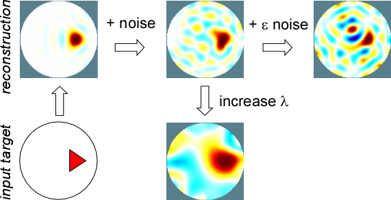
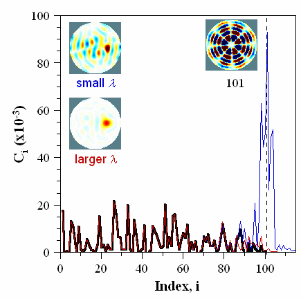
This figure shows how a larger λ results in loss of resolution. It also results in a reduction in amplitude (not shown in this figure, which did not employ normalized amplitudes). To be able to reduce the size of the hyperparameter, you must reduce noise in the signal (see below).

streching word UMD
The figure shows four reconstructions of a (simulated) triangular target. The top row of images all employ the same hyperparameter λ, with noise increasing left to right. The center figure has a level of noise that is at the upper limit of what can handled by that λ, and the rightmost figure has just a little more noise. The reconstruction on the bottom shows loss of resolution from raising λ. Recall that the EIT image is a matrix σ of conductivity changes in the sensor as a result of a touch; increases in resistance (e.g. due to strain) are here indicated in red.

Another reason for poor resolution could be

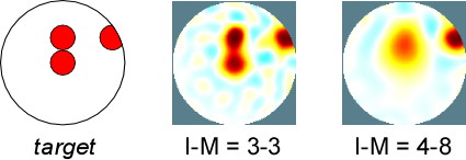
you are using a symmetric injection and/or measurement pattern (such as opposite, OP).

Some general rules of thumb regarding the I-M pattern are: never use a symmetric pattern (see the example in the figure) and for large hyperparameters avoid adjacent patterns (i.e. I-M = #-1). The overall best compromise for 16 electrodes and a circular sensor is the 3-3 pattern, but for particular imaging scenarios others may be better choices. For more information about which patterns to use, see the paper: E. Smela, "EIT for tactile sensing: considerations regarding the injection-measurement pattern," Eng. Res. Expr., 4 (4), 045041 (2022).

streching word UMD
For a 3-circle target, reconstructions made using different injection-measurement (I-M) patterns, the one on the right having high symmetry.

Recall that in EIT current is injected into some electrodes and voltages are measured at all the others. Here we consider only bipolar injection-measurement (I-M) patterns, in which current flows between two electrodes. The patterns are here numbered using the offset labeling method in which the number gives the position of the 2nd electrode relative to the first (so 1 indicates adjacent electrodes, 2 indicates that there is one electrode between them, and so on).

A third reason may be that

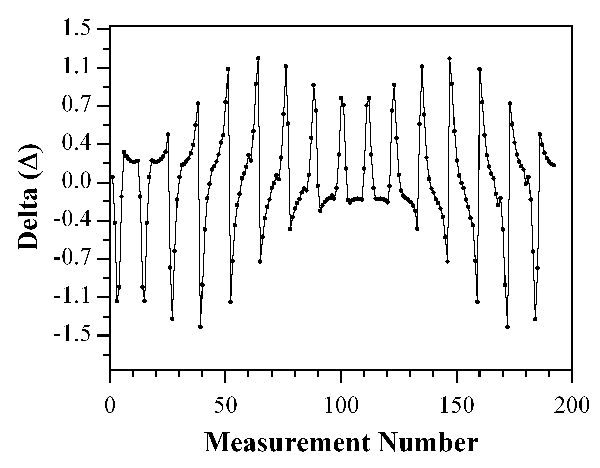
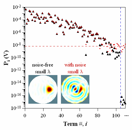
you are using a one-step algorithm instead of an iterative one.

For tactile imaging you will likely want to use a 1-step algorithm because it allows real-time operation. The default algorithm in EIDORS is the Gauss-Newton (GN) 1 -step. While iterative algorithms can give higher fidelity images, they will not give you the imaging rates you will likely need.

How should I think about noise? What is a tolerable level?

Even noise that is orders of magnitude smaller than the signal interferes with image reconstruction.

Before explaining further, let’s start by examining a typical “signal”, which is a series of voltage differences between a reference state in which the sensor is untouched and a state with a tactile contact, as shown in the figure.

streching word UMD
The signal Δ, comprising 192 measurements, in a 16-electrode system with an I-M pattern 7-1 (nearly opposite) for the triangular target shown previously. A noise level of 3x10^-7 V cannot be observed on this graph, even in a 30x close-up.

The most useful way to think about noise in EIT is in terms of Picard coefficients P_i, which can be found using EIDORS. (Our commented Matlab codes can be requested.) To understand the P_i, it is necessary to appreciate that both the signal, Δ, and the image, σ, can be expressed (via singular value decomposition, SVD) in terms of “eigen-Δ” and eigen-images. Three eigen-Δs, u_i, for 7-1 are shown in this figure.

streching word UMD
Three of the 192 total eigen-Δ , or u_i (here u₁, u₂, and u₅), for the 7-1 pattern and a circular sensor.

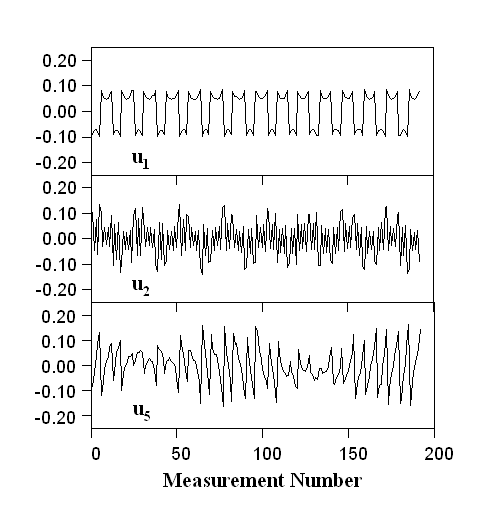
The Picard coefficients give the amplitudes, in units of V, of the u_i that sum to form the signal. This is analogous to expressing waveforms with a Fourier expansion. If there is noise on the signal, the Picard coefficients, which specify the amplitudes of these terms in the sum, are incorrect, as shown in the next figure. The larger the noise, the smaller the number of meaningful terms (carrying true image information).

streching word UMD
Picard coefficients P_i for the triangular, 7-1 example without noise (black symbols) and with noise at a level of 6x10^-9 V (red), indicated by the dashed horizontal line. There are only 104 meaningful terms in this expansion; terms above i = 104 (the rank of the Jacobian matrix, indicated by the dashed vertical line) are ignored. Note that the largest u_i, at small i, have amplitudes above 10^-3, yet the image of the triangular target is nevertheless destroyed by noise that is a million times smaller than that if the hyperparameter is too small, as shown by the corresponding EIT images.

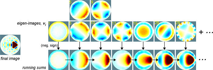
Picard coefficients P_i that are at or below the noise level add junk to the image, which must be eliminated by raising the hyperparameter. The hyperparameter is, in essence, a tunable low-pass filter that removes higher-i terms. The low-frequency information (coarse resolution) has high amplitude, but the image details (finer resolution, particularly in the center of the image) are carried in the many small-amplitude terms that are readily contaminated by noise. So, the lower the noise, the better your image fidelity can be.

How exactly is the image affected? Each u_i is linked, via singular values s_i, to an eigen-image v_i. The v_i sum to form the final conductivity change image, σ, as shown below (For illustrations of this in other contexts, see the excellent discussion by Bagheri and search online for examples of eigen-faces.)

streching word UMD
Illustration of how the triangular reconstructed image is formed from a sum of eigen-images, v_i. The several largest v_i are shown here. For a small number of terms (large hyperparameter), the resolution is poor.

Simply put, the incorrect amplitudes of the Picard coefficients correspond to incorrect coefficients C_i for the v_i in the image sum. These must be removed by raising the hyperparameter.

streching word UMD
Coefficients C_i for the eigen-images v_i for the same triangular 7-1 example. The black line indicates the C_i in the absence of noise. Large C_i resulting from the presence of noise (blue line) add higher order terms, such as the one corresponding to i = 101, resulting in the inaccurate image. A larger λ reduces the amplitudes of those terms (red line), resulting in a more correct image.

Top of Page

What hyperparameter l should I use?

In brief, the relationship between the hyperparameter and noise is linear. To determine the hyperparameter for tactile sensing, use the L-curve method. While some publications have suggested that hyperparameters given by this method are too large from the perspective of resolution (for medical imaging applications), they are optimal from the perspective of eliminating artefacts. Artefacts are the imaginary tactile contacts that appear in the image due to noise (see examples in the previous figures), which must be avoided if you are trying to detect transient tactile contacts.

It is important to understand how the hyperparameter scales with experimental variables, so that you can compare your λ with those reported by others (when they do so: some publications don’t understand EIT well enough to be aware that this parameter is important – beware of those). The table shows how λ scales with the injected current I and the baseline sensor conductivity σ₀. There should be no alteration of λ with conductivity changes Δσ (determined by the sensitivity of the sensor and the strength of the tactile contact).

Variable	Increase	Fix	For Same Effective Regularization, Change Numerical Value of λ by
I	10x	σ₀ and Δσ	increase by 10
σ₀	10x	Δσ and I	decrease by 100
Δσ	10x	σ₀ and I	no change

Top of Page

Why doesn’t increasing the number of electrodes improve resolution?

Because your hyperparameter is too large. A larger number of electrodes only helps, and then only marginally, for ultra-low noise data. This is typically unrealistic for tactile imaging applications in which you are operating in real time. (For more information about this, refer to sections in the book.) In general, there is really no benefit to using more than 12 or 13 electrodes. (The latter has the benefit of eliminating symmetry.) As always, avoid the high-symmetry I-M patterns.

Should I use a sensor with high resistance or low resistance?

In a nutshell, from the imaging perspective, high resistance if you are using constant current injection, since it will give a higher voltage signal at the measurement electrodes (since V = IR). This may pose other disadvantages, however, such as greater power consumption (P = I²R) and sensor heating (which may increase noise).

Which algorithm and prior are best?

Use the GN 1-step for its speed and use the Laplace prior for its preservation of peak “energy” (Chapter 4, section 5). The latter means that information about the overall strength of the touch has the most spatial uniformity. The peak still broadens as λ increases, with the most broadening in the center of the image, but the integral under the curve remains about the same at all positions.

Top of Page

For further information on pyEIT (as opposed to EIDORS in Matlab), see:

https://github.com/eitcom/pyEIT

Page last updated: April 16, 2024